Climate Variation Effects on Crop Yields for Maize, Soybean, Rice, and Wheat

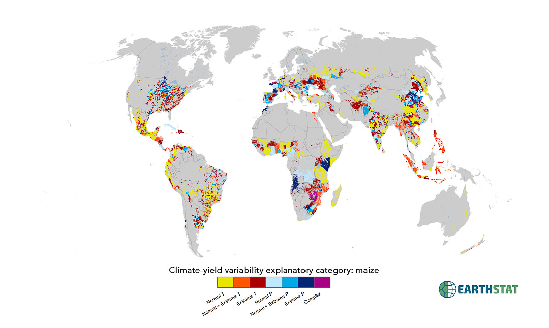
Many studies have examined the role of mean climate change in agriculture, but an understanding of the influence of inter-annual climate variations on crop yields in different regions remains elusive. We use detailed crop statistics time series for ~13,500 political units to examine how recent climate variability led to variations in maize, rice, wheat and soybean crop yields worldwide. While some areas show no significant influence of climate variability, in substantial areas of the global breadbaskets, >60% of the yield variability can be explained by climate variability. Globally, climate variability accounts for roughly a third (~32–39%) of the observed yield variability. Our study uniquely illustrates spatial patterns in the relationship between climate variability and crop yield variability, highlighting where variations in temperature, precipitation or their interaction explain yield variability. We discuss key drivers for the observed variations to target further research and policy interventions geared towards buffering future crop production from climate variability.

Citation:

Ray DK, JS Gerber, GK MacDonald, PC West. 2015. Climate variation explains a third of global crop yield variability. Nature Communications.  doi: 10.1038/ncomms6989

Contact:

Direct questions by email to earthstat.data@gmail.com

For additional information regarding publications and research, visit http://gli.environment.umn.edu/

Disclaimer:

This data does not contain unique data for each grid cell as it is aggregated based on administrative unit reporting.
This data is compiled using information gathered from individual countries’ agricultural census. The data may be accurate to country level, admin1 level or admin2 level.

Data Products:

The following data products are included:

Total crop yield variability explained due to climate variability:
(Represented by datasets with explanatorycat in title)

1. No Effect;
2. 0 to 0.15;
3. 0.15 to 0.30;
4. 0.30 to 0.45;
5. 0.45 to 0.60;
6. 0.60 to 0.75;
7. greater than 0.75

Resolution:

Spatial: Five minute by five minute resolution (~10km x 10km at equator)

Map Projection:

• Data presented as five-arc-minute, 4320 x 2160 cell grid
• Spatial Reference: GCS_WGS_1984
• Datum: D_WGS_1984
• Cell size: 0.083333 degrees
• Layer extent:
  • Top : 90
  • Left: -180
  • Right: 180
  • Bottom: -90

License:

Creative Commons Attribution 4.0 International

Data may be freely downloaded for research, study, or teaching, but must be cited appropriately.  Re-release of the data, or incorporation of the data into a commercial product, is allowed only with explicit permission.  If you would like to request permission to use EarthStat data for another purpose, please contact us at earthstat.data@gmail.com.

Methods:

From Ray et al. 2012:

Modelling set-up
Further details regarding the data used are given in Supplementary Methods 1. To determine how much of the variability in crop yields was explained by climate variability, we first detrended the crop yield and climate variables—temperature and precipitation—following1 (see the example in Supplementary Fig. 7) over the period 1979–2008. Note that we use two forms of temperature and precipitation—the seasonal or growing season average value and the average conditions 12 months before harvest or the annual value to account for antecedent conditions. This resulted in four different combinations of detrended climate variables, and as we used both the linear and squared forms of seasonal and annual temperature and precipitation there was a total of eight forms of climate variables. We used these detrended variables in different combinations to linearly regress with the detrended crop yields at each of the 13,500 political units. To avoid over-fitting we limited our analysis to a total of 27 combinations of climate variables, resulting in 27 regression equations, to capture the relationships between climate variability and crop yield variability at each political unit and of the basic form:

Yc = f(Tc, Pc )   (1)

where Yc is the observed set of detrended crop yields for crop ‘c’ in units of tons/ha/year at each political unit; In equation 1, Tc can represent for crop ‘c’ at a given political unit the temperature associated with the main growing season64 or the temperature for 1 year before the crop’s harvest to capture antecedent conditions. Pc similarly is the precipitation for the main growing season for the crop ‘c’ for the political unit and for 1 year before the crop’s harvest. The function f is limited to linear and quadratic forms of these two detrended meteorological parameters, as is common practice in studies correlating climate and agricultural production. The terms included in each of the 27 regression equations and their classification are provided in the Supplementary Table and further details are given in Supplementary Methods 2.

Statistical tests
The generated regression equations at each political unit, for example, ~13,500 sets of 27 equations per crop, were statistically tested next. We first identified which functional form of Yc=f(Tc, Pc) from the set of 27 equations at each political unit fit the data best using the Akaike Information Criterion (AIC), which penalizes equations with more terms. However, because the model that best fits the data may be no better than a random climate (null model), we conducted F tests at the P=0.10 level to determine whether the chosen model was significantly better than the null model. In 21–47% of the global crop-harvested areas, we found that the chosen model was no better than the null model at the P=0.10 significance level. Thus, in the remainder 53–79% of global crop harvested areas yield variability is significantly influenced by climate variability over the study period and our reported numbers are averages over these areas.

Using the statistically significant model with the best functional representation, we next determined the coefficient of determination (r2) or explanatory power of the complete model, and the reduced models containing only temperature and only precipitation terms. The residual is the unexplained yield variations.

The 30-year study period average harvested area and yield information at each subnational location was used together with the observed coefficient of determination for computing national and global harvested areas weighted averages. Global and country-specific numbers are averaged only over those 53–79% of global crop harvested areas where the statistical models were significant.

Model bias and sensitivity
As a simple assessment of model bias, we performed a bootstrapping exercise to assess the influence of including specific combinations of years (80% of the years selected at each iteration) in our data on the overall yield predictions (using a test set of 20% of the years) for each political unit, which we standardized as the ratio of the average bias from the 99 repetitions to the average of the crop yields for the study period in each political unit (Supplementary Fig. 8). This is analogous to a leave-group-out cross validation approach used to examine uncertainty in model selection. Locations of models with more restrictive P cutoff values (F-tests) at P=0.01 and P=0.05 are shown in Supplementary Fig. 9. In general, even though we used a less-restrictive P-value of 0.1, the models selected generally were significant at P=0.05 or less.