Yield Gaps and Climate Bins for Major Crops

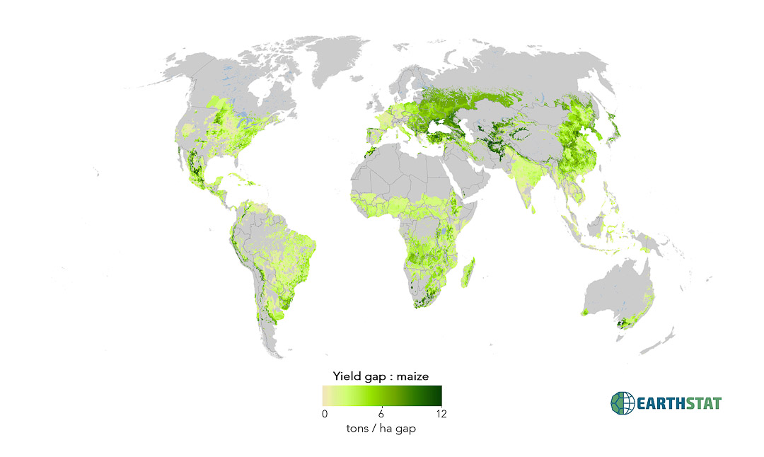
Large yield variations exist across the world, even among regions with similar growing conditions, suggesting the existence of ‘yield gaps’. Here we define a yield gap as the difference between observed crop yields and the attainable yield at the same location. It is estimated that bringing the world’s yields to within 95% of their attainable yield for 16 important food and feed crops could increase current production by 58%.  We use the term ‘attainable yield’ to differentiate from agronomic potential – which represents a higher yield ceiling which may not be economically feasible.  Yield gaps were estimated by comparing observed yields to attainable yields determined by identifying high-yielding areas within zones, or bins, of similar climate.

Citation:

Mueller, N. D., Gerber, J. S., Johnston, M., Ray, D. K., Ramankutty, N., & Foley, J. A. (2012). Closing yield gaps through nutrient and water management. Nature, 490, 254. doc: 10.1038/nature11420

Contact:

Direct questions by email to earthstat.data@gmail.com or navin.ramankutty@ubc.ca

For additional information regarding publications and research, visit http://gli.environment.umn.edu/ or http://www.ramankuttylab.com

Data Products:

The following data products are included for each of 16 major crops:

• Yield Gaps – tons per hectare gap
• These data represent the average yield gap between observed yields in the year 2000 and an attainable yield derived from comparison to other farmers growing that crop in areas of similar climate.
• Potential or attainable yields – tons per hectare
• These data represent the highest yield obtained by farmers growing that crop in areas of similar climate. The attainable yield in this case is the 95^th percentile value of reported yields in a similar climate space.
• Climate Bins – defined by precipitation and growing degree days in crop area
• For each crop, individual climate bins cover equal harvested areas. For a more detailed discussion on how crop area was binned, see Mueller et al.

Resolution:

• Spatial: Five minute by five minute resolution (~10km x 10km at equator)
• Temporal: Year 2000 – Average of census data between 1997-2003

Map Projection:

• Data presented as five-arc-minute, 4320 x 2160 cell grid
• Spatial Reference: GCS_WGS_1984
• Datum: D_WGS_1984
• Cell size: 0.083333 degrees
• Layer extent:
  • Top : 90
  • Left: -180
  • Right: 180
  • Bottom: -90

License:

Data may be freely downloaded for research, study, or teaching, but must be cited appropriately.  Re-release of the data, or incorporation of the data into a commercial product, is allowed only with explicit permission.  If you would like to request permission to use EarthStat data for another purpose, please contact us at earthstat.data@gmail.com.

Methods:

While there are multiple ways in which climate can be classified, we followed the logic of Prentice et al. (1992), who described relationships between climate and global biomes. We used two parameters known to be fundamental drivers of plant growth to describe a region’s climate – growing degree days (GDD) and a crop soil moisture index (the ratio of actual evapotranspiration to potential evapotranspiration).

We calculated GDD as in Ramankutty et al. (2002), with

GDD = i=1365max(0,Ti-Tb)days-degrees

where Ti is the temperature in °C at each time step and Tb is a crop-specific baseline temperature. For those crops generally grown in warmer climates (cassava, cotton, groundnut, maize, millet, oil palm, sorghum, soybean, sugarcane and sunflower), we used a Tb of 8 °C, whereas we used a Tb of 2 °C for those crops also found in cooler regions (potato, pulses, rapeseed, rye and sugarbeet). We use an observed Tb of 0 °C for wheat, 1 °C for barley and 5 °C for rice.

We then calculated the crop soil moisture index as the ratio of actual evapotranspiration to potential evapotranspiration (AET/PET), similar to Prentice et al. (1992) and Ramankutty et al. (2002). Building on methodology developed in Zaks et al. (2007), we created a 10 ¥ 10 matrix of GDD and average, annual crop soil moisture availability with 100 different climate zone combinations.  For each axis of the matrix, we divided the GDD and crop soil moisture index data, respectively, into 10 equal parts. For example, because the crop soil moisture index data ranged from 0 to 1, the bounds of soil moisture in the first ‘bin’ of the matrix were 0 and 0.1. For a crop like wheat with a baseline temperature of 0 °C, because the maximum number of growing degree days above 0 °C on Earth is approximately 11,168, the bounds of GDD for the first bin were approximately 0 and 1117 days; the number of GDD per bin varied depending on the baseline temperature used. We then assigned each grid cell to one of the 100 climate zones, based on its GDD and crop soil moisture conditions.

We subsequently distributed the yields from each grid cell, crop by crop, into their respective climate zones. By doing so, we obtained a distribution of yields for each crop in each climate zone. To ensure that we had a statistically meaningful number of yield observations in each climate zone, we imposed a five data point threshold for the yield distributions. If there were not yield observations from at least five different grid cells, we did not include the climate zone for that crop in our analysis. However, the number of observations in each climate zone distribution varied depending on the climate each crop is typically grown in. For example, oil palm is typically grown in warm, humid climates; there were few to no observations in other climate zones.

For each climate zone and each crop we generated a table containing the yield, harvested area and latitude/longitude position information for each grid cell included in the distribution. We then sorted the data from the grid cells by their yield values, ranking them from lowest yield to highest. Next, starting with the grid cell with the lowest yield value, we accumulated the grid cells’ respective harvested areas, until we arrived at the statistical information of interest: the mean, median and 90th percentile yields. We then used the respective yield data from that point to define the mean, median and 90th percentile yields. (Other statistical properties, such as the 25th and 75th percentile yields can also be calculated with this method.) With this approach, we defined a percentile yield value by accumulating that percentage of a crop’s harvested area, rather than that percentage of a crop’s yield observations. This allowed us to prevent grid cells with smaller amounts of cultivation from skewing the results.